This is one of the most questioned topics in Data Science interviews and one of the simplest methodologies to understand when starting to learn Machine Learning. Let’s finally understand what Gradient Descent is really all about!
According to Aurélien Géron’s book “Hands on Machine Learning with Scikit-Learn & TensorFlow” (great book, for who is starting):
Gradient Descent is a very generic optimization algorithm capable of finding optimal solutions to a wide range of problems. The general idea (…) is to tweak parameters iteratively in order to minimize a cost function.
Before we go further into explaining in more detail Gradient Descent, it is important to understand what is a Cost Function.
What is a Cost Function?
Let’s start this terminology by taking the simplest example of a Machine Learning algorithm: Linear Regression. Linear Regression is used to estimate linear relationships between continuous or/and categorical data and a continuous output variable.
//[ \hat{y} = \theta_0 + \theta_1 x_1 + \theta_2 x_2 + … + \theta_n x_n]//
- y^ is the predicted value
- n is the number of features
- xi is the ith feature value
- θj is the jth model parameter (including the bias term θ0 and the feature weights θ1, θ2, ⋯, θn).
To make things simpler, we’ll assume a practical example. You can imagine that our predicted value y is sales while X is advertising spends. We want to create a model that can estimate how the advertising budget impacts sales.
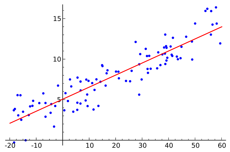 Our linear model (red) generalising to all the data available (blue dots). Wikipedia
Now, what our model tried to best estimate the parameter θj that would generalise for future advertising budget data, allowing us to make good predictions on the sales return. Cost Functions are used to measure how wrong the model is in terms of its ability to estimate the relationship between our advertising budget X and our target variable, sales y. Usually, the cost function is described as the difference between the predicted value given by our model and the true value.
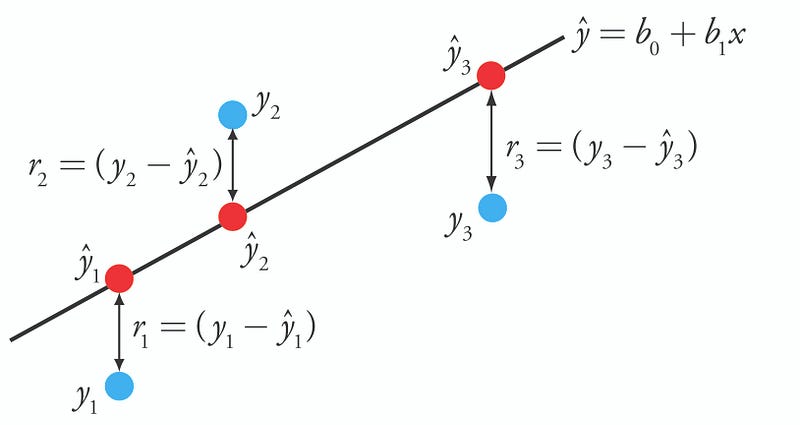 Difference or distance between the predicted value (red) and the actual value (blue).
Therefore, the goal of a Machine Learning algorithm is to find the best parameters θj which will minimise the cost function.
Gradient Descent:
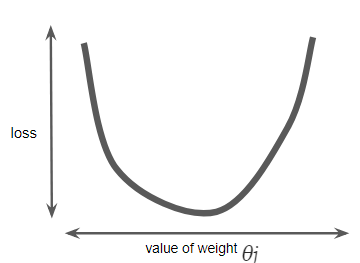
Minimising the Cost Function Hopefully, you’re now more enlightened on what is a cost function and we can go on explaining why gradient descent is so important. As previously said, gradient descent is an efficient optimisation algorithm that attempts to find the global minima of a cost function. According to Aurélien, the gradient descent “measures the local gradient of the error function with regards to the parameter vector θj, and it goes in the direction of descending gradient. Once the gradient is zero, you have reached the minimum.” For most regression problems, the resulting plot of “Cost Function vs Parameter θ” will always be convex therefore having only a single minimum where the slope is exactly zero and also where the cost function converges.
Calculating the cost function parameters for all θj over the entire data set would be an inefficient way of finding the convergence point. This is where gradient descent does its magic! But how does it work?
You start by randomly fill the parameter θ with random values (also known as random initialisation). At this point, the gradient descent algorithm calculates the gradient of the loss curve at the starting point, which is the derivative (slope) of the curve. In the end, it gives you the direction of your next step.
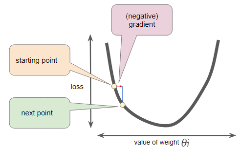
You repeat this process incrementally, each step at a time, trying to reduce the cost function until your algorithm converges to a minimum as shown in this gif below.
 Cost Function vs Value of Weight (parameter θ).
At this point (local minimum) the model has optimised the parameters such that it minimise to a minimum the cost function.
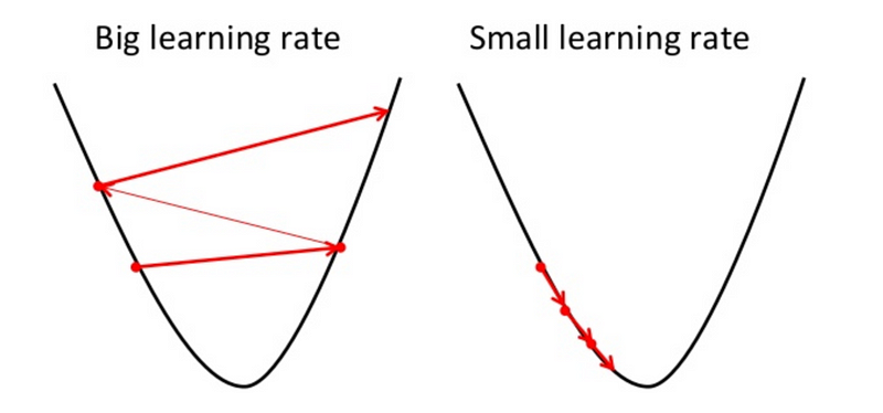
Importance of the Learning Rate
We’ve seen so far that the gradient vector has both a direction and a magnitude (red arrow). The gradient descent algorithm multiplies the gradient by a scalar known as learning rate (or step size). Hence, the learning rate is the hyperparameter that the algorithm uses to converge either by taking small steps (much more computational time) or larger steps. See the following gif examples to understand the impact of selecting different learning rates.
Learning rate = 0.10
Learning rate = 1.0
Learning rate = 1.6 
The examples show great learning rates that allowed us to achieve the cost function convergence point slower or faster. Nevertheless, just be careful when choosing higher learning rates since this might take the algorithm to diverge, with larger and larger values, failing to find a good solution. Take a look at the image below for an example.
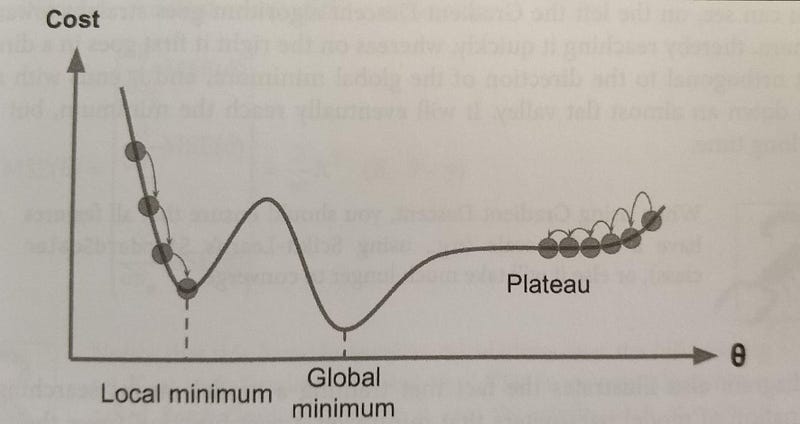
Moreover, you should also have in mind that not all cost functions look like nice regular bowls. That usually happens for Linear Regression, and it is great because regardless of your initial assumption for parameter θj it will always converge. With other Machine Learning algorithms such as Neural Networks you might find cost functions with irregularities making it hard to converge.
Take into consideration the image below. If our random initialisation for our parameter θj starts on the left our algorithm will converge to a minimum which is not the best. However, if it starts on the right it will take longer to do the plateau and eventually might reach the right minimum if you do not stop early
An important fact you should have in mind is that all features should have similar scales in order to ensure the algorithm will not take more than necessary to converge.
The types of Gradient Descent
There are three popular gradient descent types that mainly differ for the amount of data they handle.
Batch Gradient Descent
In gradient descent, the batch is the total number of examples you use to calculate the gradient in a single iteration. This algorithm does its calculations over the full training dataset, at each step of the gradient descent. Hence, it uses the whole dataset at every step, making it very very very slow for large datasets.
Pros: Computational efficient, since it produces a stable error gradient and a stable convergence.
Cons: Requires that the training dataset is in memory and available to the algorithm. It is slow since it uses the whole training set to compute the gradient at every learning step.
Stochastic Gradient Descent
This alternative to Batch Gradient Descent, it is on the other extreme of the idea, using a single example (batch of 1) per each learning step. Of course, due to this methodology ,the algorithm is much faster since it has few data to manipulate at every iteration, however it can return very noisy gradients which can cause the error rate to jump around. Therefore, due to this jumping around when the algorithm stops instead of finding the optimal fit it ends up obtaining only good results.
Pros: Constant update allows us to have a detailed rate of improvement. Allows usage of huge datasets since only one instance is needed to be allocated to the memory at each step.
When the cost function is very irregular such as in the last image, due to the jumping around this algorithm behaves better.
Cons: Due to its stochastic (i.e. random) nature, the algorithm is much less regular than the previous one. Instead of slowly decreasing the cost function until it reaches the desired value, the Stochastic bounces up and down only decreasing on average. Jumping around is good to escape local minimum but bad because hardly the algorithm will ever settle at the global minimum.
Mini Batch Gradient Descent
This is the go-to method! Contrary to the two last gradient descent algorithms that we saw, instead of using the full dataset or a single instance, the Mini Batch, as the name indicates ,computes the gradients on small random sets of instances called mini batches.
This algorithm is able to reduce the noise from the Stochastic and still be more efficient than full-batch. Basically, it splits the training dataset into small batches ranging from 10 to 1,000 examples, chosen at random.
This algorithm is the best option when you are training a neural network and it is the most common within the Deep Learning field.
Resources :
- Hands-on Machine Learning with Scikit-Learn & TensorFlow by Aurélien Géron
- Google’s Machine Learning Crash Course